Three myths about quantum computing — Part 3: Teleportation and superdense coding

This is the last post in the series on myths about quantum computing.

One of the most exciting things about quantum information is quantum teleportation—the ability to transmit quantum data by sending only classical bits. Superdense coding is another surprising protocol which lets you transmit two classical bits by sending only one qubit.

It is often mistakenly believed that these two features of quantum information do not have a classical equivalent. The goal of this post is to explain why this is not the case, and to clarify other related misconceptions.

Bell states

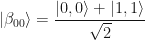
Let us first briefly discuss some simple facts that are useful for explaining how quantum teleportation works. Let $z, x \in \{0,1\}$ . Then the following four two-qubit states are orthonormal and form a basis:

$|\beta_{zx}\rangle = \dfrac{|0,x\rangle + (-1)^z |1,\bar{x}\rangle}{\sqrt{2}}$

This is known as Bell basis. One can prepare $|\beta_{zx}\rangle$ from the standard basis state $|z,x\rangle$ as follows:

$|\beta_{zx}\rangle = \mathrm{CNOT} \cdot (H \otimes I) \cdot |z,x\rangle$

One of the most important properties of Bell states is that any Bell state can be mapped to any other by applying local Pauli matrices on only one of the systems:

$|\beta_{zx}\rangle = (Z^z X^x \otimes I) \cdot |\beta_{00}\rangle = (I \otimes X^x Z^z) \cdot |\beta_{00}\rangle$

Quantum teleportation

The setting for quantum teleportation is as follows. Assume that Alice has a single-qubit quantum state $|\psi\rangle$ that she wants to send to Bob. Moreover, they have met beforehand and established a joint two-qubit quantum state

$|\beta_{00}\rangle = \dfrac{|0,0\rangle + |1,1\rangle}{\sqrt{2}}$

known as EPR pair, shared between them. Here is a schematic diagram of how quantum teleportation works:

Here “Bell” denotes the measurement in the Bell basis whose outcomes are classical bits z and x, and $Z^z X^x$ is the correction operator that Bob has to apply to recover the original state.

Quantum teleportation works because of the following identity:

$|\psi\rangle \otimes |\beta_{00}\rangle = \displaystyle \frac{1}{2} \sum_{z,x \in \{0,1\}} |\beta_{zx}\rangle \otimes X^x Z^z |\psi\rangle$

which holds for any single qubit state $|\psi\rangle$ . From this identity we see that when Alice performs the Bell measurement, she gets two uniformly random bits z and x, and Bob’s state collapses to $X^x Z^z |\psi\rangle$ which is a distorted version of $|\psi\rangle$ . Once Bob receives z and x, he can apply $Z^z X^x$ to recover $|\psi\rangle$ . Note that an adversary who intercepts z and x cannot learn anything about $|\psi\rangle$ , since both bits are uniformly random.

The usual argument why quantum teleportation is surprising, is that it allows to transmit a quantum state $|\psi\rangle$ with two continuous degrees of freedom (say, the angles in the Bloch sphere) by sending only two classical bits. This may seem quite paradoxical, since it appears as if two real numbers have been transmitted by sending just two bits. However, this is not the case at all, since the two parameters describing $|\psi\rangle$ cannot be recovered (to any reasonable degree of precision) from a single copy of $|\psi\rangle$ . For example, we know by Holevo’s theorem that one cannot learn more than one bit of information by measuring $|\psi\rangle$ .

Classical teleportation

What is the classical equivalent of the above procedure? Let us first set up some terminology and notation. Since we will be dealing with probability distributions, let

$\mu = \dfrac{1}{2} [0] + \dfrac{1}{2} [1]$

denote the uniform distribution over {0,1}. Similarly, let

$\beta = \dfrac{1}{2} [0,0] + \dfrac{1}{2} [1,1]$

be the classical version of the EPR state $|\beta_{00}\rangle$ .

Intuitively, one should think of probability distributions as a way of describing a coin that has been flipped and (without looking at it) put inside a sealed envelope. Note that one can perform operations on such coin, even though its exact state is not known. For example, by flipping the envelope around one can perform the logical NOT. One could also imagine some more complicated procedures for performing joint operations on two coins in a joint unknown state.

We will use the term pbit to refer to a probabilistic bit that describes a coin inside the envelope. Note that a pbit has one degree of freedom. However, once the envelope has been opened, the state of the coin becomes certain, i.e., either [0] or [1], so we will describe it by a deterministic bit or dbit. Note that this is analogous to how measurements work in the quantum case, except that in the classical case there is only one measurement basis—the standard basis.

Now we are ready to describe the classical teleportation. Our task is the following: we would like to transmit one pbit by sending one dbit. In other words, we want to transmit one degree of freedom per one classical bit being sent, just as in the quantum case.

At first, this might seem trivial—can’t we just send the bit over and be done? Unfortunately, not. Recall that we want to transmit a pbit or an “unobserved coin”, but we are allowed to send only a dbit. In other words, your envelope will always be opened and its content revealed, just as if you were a journalist sending an e-mail from China. Let us depict this situation with the following diagram:

Here the dark pipe represents a pbit in state $\pi$ , but the white pipe a dbit obtained by observing $\pi$ . The dashed line between Alice and Bob represents Chinese government.

To make this scheme work, we will use a shared resource between Alice and Bob as in the quantum case. A natural classical equivalent of the EPR state $|\beta_{00}\rangle$ is the probability distribution $\beta$ defined above. To preserve our pbit $\pi$ , we will XOR it with Alice’s half of $\beta$ , and send the result over to Bob. Even though the pbit $\pi$ is turned into a dbit due to Chinese government spying on Alice, Bob can still XOR it with his half of $\beta$ and recover the original pbit $\pi$ :

This indeed gives the correct result, since the original pbit essentially gets XORed with the same value twice. Intuitively, one can think of it being transmitted “back in time” through the black pipe that represents $\beta$ . Just as in the quantum case, the party who intercepts the transmitted bit learns nothing about $\pi$ , since the transmitted bit is uniformly random. In fact, this scheme is equivalent to one-time pad.

Quantum superdense coding

Quantum superdense coding is the dual protocol of quantum teleportation (this can be made more precise by considering coherent communication). It allows to send two classical bits by transmitting a single qubit and consuming one shared EPR pair.

Initially Alice and Bob share an EPR state $|\beta_{00}\rangle$ . Alice encodes her two classical bits z and x in her half of $|\beta_{00}\rangle$ by performing $Z^z X^x$ . This maps the joint state of Alice and Bob to Bell state $|\beta_{zx}\rangle$ as discussed above. Then Alice sends her qubit over to Bob, who can recover both bits by performing a measurement in the Bell basis:

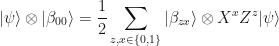
Quantum superdense coding works because of the following identity:

$(H \otimes I) \cdot \mathrm{CNOT} \cdot (Z^z X^x \otimes I) \cdot |\beta_{00}\rangle = |z,x\rangle$

This immediately follows from the properties of Bell states discussed above. Since all Bell states are maximally entangled, their reduced states are completely mixed, so the transmitted qubit contains no information about the two encoded classical bits z and x.

Classical “supersparse” coding

Classical superdense coding is very similar to classical teleportation, except the roles of dbit and pbit are reversed, i.e., Alice wants to transmit a dbit by sending a pbit. This seems to be even simpler than teleportation, since we are given more resources and asked to perform a simpler task! In fact, there is nothing “superdense” about this task, as it only wastes resources. In this sense it would be more appropriate to call it “supersparse” coding!

The only catch is that for complete analogy with the quantum case, the transmitted pbit should be uniformly random, so that a potential eavesdropper could learn nothing about the original message. Here is a protocol that achieves the task of transmitting a dbit b in the desired way:

Note that the only difference between this picture and the one for classical teleportation is the color of pipes.

Conclusion

Quantum teleportation should not seem more surprising than the classical one, since in both cases one degree of freedom is transmitted per one classical bit being sent. The only quantitative difference is a factor of two in the amount of resources consumed: one ebit is consumed for sending two degrees of freedom in the quantum case versus one shared random bit per single degree of freedom in the classical case. Recall that we observed the same factor-of-two difference in the case of the amount of information needed to specify a quantum versus a classical probabilistic state within the exponential state space.

Thus, given the existence of a classical equivalent, quantum teleportation should not seem too surprising. At least, no more than by a factor of two!

p.s. As Matthew Leifer has pointed out to me, these and many other analogies between quantum entanglement and secret classical correlations have been described in the paper “A classical analogue of entanglement” by Daniel Collins and Sandu Popescu.

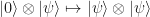
Three myths about quantum computing — Part 2: No-cloning theorem

Posted by Māris Ozols

This is the second post in the series on myths about quantum computing.

One of the first things we learn about quantum information is that it cannot be copied. This may seem rather surprising and counter-intuitive, since classical information stored on your computer can be easily copied (in fact, it is extremely challenging to come up with methods that would prevent this). One might even conclude that there must be something special about quantum information that does not allow us to copy it.

My goal in this post is to argue that this is not the case. The main point is that classical probability distributions cannot be copied either. This observation should make the quantum no-cloning theorem seem less surprising.

Quantum no-cloning theorem

Let us consider the standard argument why quantum states cannot be copied—the main idea is that unitary transformations have to preserve inner products.

Theorem 1 (Quantum no-cloning theorem). Transformation that acts as

$|0\rangle \otimes |\psi\rangle \mapsto |\psi\rangle \otimes |\psi\rangle$

for any quantum state $|\psi\rangle$ , is not unitary.

Proof. Let $|\psi_1\rangle$ and $|\psi_2\rangle$ be two quantum states, and assume that U is a unitary operation that implements the desired transformation. Then

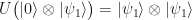
$U \bigl( |0\rangle \otimes |\psi_1\rangle \bigr) = |\psi_1\rangle \otimes |\psi_1\rangle$

$U \bigl( |0\rangle \otimes |\psi_2\rangle \bigr) = |\psi_2\rangle \otimes |\psi_2\rangle$

If we take the inner product of the corresponding sides of these two equations, we get

$\langle\psi_1|\psi_2\rangle = \langle\psi_1|\psi_2\rangle^2$

where we used the assumption that U is unitary. When we solve this, we get that either $\langle\psi_1|\psi_2\rangle = 0$ or $\langle\psi_1|\psi_2\rangle = 1$ . This means that using a unitary transformation we can only copy states from an orthonormal set. However, the set of all quantum states is not orthonormal, so there is no unitary transformation that would copy an arbitrary unknown quantum state. $\blacksquare$

Classical no-cloning theorem

Recall from the previous post that quantum states and classical probability distributions are not that much different. Let us see if we can come up with a no-cloning argument that would also work in the classical case.

First, observe that independent probability distributions are combined in exact same way as quantum states—using the Kronecker product. (There is nothing “quantum” about the $\otimes$ operation!) In probabilistic classical computing the set of allowed transformations are those that map probability distributions to probability distributions. Such transformations are called stochastic. In general, they do not preserve inner products, so our previous argument will not go through.

Let us consider an alternative argument, based on linearity. For simplicity, let us consider only probability distributions over {0,1}.

Theorem 2 (Classical no-cloning theorem). Transformation that acts as

$\begin{pmatrix} 1 \\ 0 \end{pmatrix} \otimes \pi \mapsto \pi \otimes \pi$

for any probability distribution $\pi$ , is not stochastic.

Proof. Let

$\pi = \begin{pmatrix} p \\ q \end{pmatrix}$

be an arbitrary probability distribution over {0,1}. We would like to have a stochastic operation that implements the transformation

$\begin{pmatrix} p \\ q \\ 0 \\ 0 \end{pmatrix} \mapsto \begin{pmatrix} p^2 \\ pq \\ qp \\ q^2 \end{pmatrix}$

for any p and q. However, this is not possible, since the above transformation is clearly not linear. $\blacksquare$

Note that the only property we needed in this proof was linearity, so one can use exactly the same argument also for the quantum case.

Three myths about quantum computing — Part 1: Exponential size state space

Posted by Māris Ozols

This is the first post in the series on myths about quantum computing. In this post I will discuss the first misconception about quantum computers—that the exponential size of their state space is the main feature that distinguishes them from their classical cousins—and explain why this should not be used as an argument to suggest that quantum computers are likely to be more powerful than the classical ones.

Consider a system S with states labelled by n-bit strings. Assume that S is initialized in all-zeroes state “00…0” and undergoes some kind of physical evolution. Let us consider three scenarios.

Deterministic classical world

If the evolution is deterministic, then one can specify the current state of the system by giving the corresponding label. Thus, one needs n bits of information to describe the state in this case.

Quantum world

If S is a quantum system, it can be in a superposition of all possible states. To describe this superposition, one has to assign a complex number to each state. Thus, in total one has to specify 2ⁿ complex numbers (say, to some finite precision), which is exponentially more information than in the deterministic case!

If you have never heard of this before (or remember your excitement when you heard it the first time), this definitely is mind-boggling. In fact, this is often mentioned as the main obstacle for efficiently simulating quantum computers, and also as a hand-waving argument to convince wider public that quantum computers are likely to be exponentially more powerful than classical ones.

Probabilistic classical world

One should not get too excited about the above observation, but instead think more carefully whether this comparison of deterministic and quantum computers is fair. Since the output of a quantum computer is intrinsically probabilistic, one should be looking at probabilistic evolution in the classical case, not deterministic.

If the transitions between states of the system S are described by probabilities, then the resulting state is a probability distribution over {0,1}ⁿ. To describe such distribution, one needs to specify 2ⁿ real numbers—one for each n-bit string. This is also exponentially more information than in the deterministic case!

Thus, with this comparison the only difference in the amount of information needed to describe classical and quantum states is a factor of two (since probability can be specified by a single real number whereas two real numbers are needed to specify one complex quantum amplitude).

Conclusion

The fact that an exponential amount of information is needed to describe the state space of a particular computational model does not immediately imply that it is exponentially more powerful. To be more specific, let us consider the classes of decision problems that can be solved in polynomial time by the three computational models discussed above:

The following inclusions are trivial:

$\mathrm{P} \subseteq \mathrm{BPP} \subseteq \mathrm{BQP}$

However, as of now, none of these inclusions is known to be strict.

Thus, one should not use the exponential size of the state space as an argument to claim that quantum computers are likely to be hard to simulate by deterministic classical computers, since the same argument could also be used in favor of probabilistic classical computers.

To me it seems that the main difference between probabilistic and quantum computers is the underlying field of numbers (non-negative real numbers versus complex numbers). It is a major open problem to show if this subtle difference can be used to separate the corresponding two complexity classes.

Three myths about quantum computing

Posted by Māris Ozols

In this series of posts I will discuss some misconceptions about quantum computing.

One often hears people saying that quantum physics is “strange” and that our classical intuition “breaks down” in the quantum world. I will try to argue that one should not brag about the weirdness of quantum mechanics without carefully investigating the corresponding phenomena in the classical world. In fact, many quantum phenomena no longer seem surprising once their lesser cousins in the classical probabilistic world are understood.

To illustrate my point, I will consider three basic properties of quantum information

and discuss how they translate to the classical case.

These topics are usually covered in the first class of an introductory quantum computing course, so none of what I discuss should come as a surprise to somebody who has taken such a course or read an introductory textbook on the topic. However, I have to admit that I was equally shocked both, when I learned these basic facts about quantum information in class, as when I later realized that they have a corresponding classical counterpart.

I would like to acknowledge all my “non-quantum” friends with whom I have had conversations about quantum physics. I would probably still believe in these misconceptions if I had not tried to explain you in simple terms why quantum physics is supposed to be so strange. Maybe it is not so strange after all…

p.s. For those of you who have never attempted to explain what you are doing to somebody who does not have a PhD degree in your area of expertise, consider the following three quotes by the founders of quantum mechanics:

Most of the fundamental ideas of science are essentially simple, and may, as a rule, be expressed in a language comprehensible to everyone.
—Albert Einstein

The physicist may be satisfied when he has the mathematical scheme and knows how to use it for the interpretation of the experiments. But he has to speak about his results also to non-physicists who will not be satisfied unless some explanation is given in plain language. Even for the physicist, the description in plain language will be the criterion of the degree of understanding that has been reached.
—Werner Heisenberg

If you cannot—in the long run—tell everyone what you have been doing, your doing has been worthless.
—Erwin Schrödinger

Unitary equivalence of purifications

Posted by Māris Ozols

Purifications

Let $\rho$ be a mixed quantum state on system $\mathcal{A}$ . We say that a pure quantum state $|\psi\rangle$ on a composite system $\mathcal{A} \otimes \mathcal{B}$ is a purification of $\rho$ if

$\rho = \mathrm{Tr}_B (|\psi\rangle \langle\psi|)$

The following theorem is a basic result in quantum information theory.

Theorem 1 (unitary equivalence of purifications). If $|\psi\rangle$ and $|\phi\rangle$ are two purifications of $\rho$ then

$|\phi\rangle = (I_A \otimes U) |\psi\rangle$

for some unitary $U$ that acts only on system $\mathcal{B}$ .

Schmidt decomposition

The above result is usually proved using the following theorem.

Theorem 2 (Schmidt decomposition). Any bipartite quantum state $|\psi\rangle$ on $\mathcal{A} \otimes \mathcal{B}$ can be written as

$|\psi\rangle = \sum_i \sqrt{p_i} |\alpha_i\rangle |\beta_i\rangle$

for some orthonormal bases $\{|\alpha_i\rangle\}$ and $\{|\beta_i\rangle\}$ on systems $A$ and $B$ , respectively, and a probability distribution $\{p_i\}$ .

However, standard proofs of Theorem 1 are often based on the following (wrong) argument: given two spectral decompositions of the same matrix, the corresponding eigenvalues and eigenvectors in both decompositions must be equal. This is true only if the given matrix has a non-degenerate spectrum. Otherwise the eigenvectors corresponding to a repeated eigenvalue are not uniquely determined (any orthonormal basis of the corresponding subspace is a valid set of eigenvectors).

A simple proof of Theorem 1

Here is an elementary proof of Theorem 1 which does not run into problems in case of a degenerate spectrum. By Theorem 2 we can write the first state as

$|\psi\rangle = \sum_i \sqrt{p_i} |\alpha_i\rangle |\beta_i\rangle$

Let us expand the first register of the second state $|\phi\rangle$ in the basis $\{|\alpha_i\rangle\}$ :

$|\phi\rangle = \sum_i |\alpha_i\rangle |\tilde{\gamma}_i\rangle$

where $\{|\tilde{\gamma}_i\rangle\}$ are some arbitrary (non-normalized) vectors. Then we have

$\mathrm{Tr}_B (|\psi\rangle \langle\psi|) = \sum_{i,j} \sqrt{p_i p_j} |\alpha_i\rangle \langle\alpha_j| \mathrm{Tr} (|\beta_i\rangle \langle\beta_j|)$

$= \sum_{i,j} \sqrt{p_i p_j} |\alpha_i\rangle \langle\alpha_j| \delta_{ij}$

and

$\mathrm{Tr}_B (|\phi\rangle \langle\phi|) = \sum_{i,j} |\alpha_i\rangle \langle\alpha_j| \mathrm{Tr} (|\tilde{\gamma}_i\rangle \langle\tilde{\gamma}_j|)$

$= \sum_{i,j} |\alpha_i\rangle \langle\alpha_j| \langle\tilde{\gamma}_j|\tilde{\gamma}_i\rangle$

By assumption, both partial traces are equal. Since $\{|\alpha_i\rangle\}$ is an orthonormal basis, the coefficients in both expressions must be the same:

$\sqrt{p_i p_j} \delta_{ij} = \langle\tilde{\gamma}_j|\tilde{\gamma}_i\rangle$

This means that $|\tilde{\gamma}_i\rangle$ are pairwise orthogonal and $\||\tilde{\gamma}_i\rangle\| = \sqrt{p_i}$ (it could happen that $p_i = 0$ for some $i$ , but this is not a problem). Equivalently, this equation says that we can find an orthonormal basis $\{|\gamma_i\rangle\}$ such that $|\tilde{\gamma}_i\rangle = \sqrt{p_i} |\gamma_i\rangle$ . Then we see that $|\phi\rangle = (I \otimes U) |\psi\rangle$ , where $U = \sum_i |\gamma_i\rangle \langle\beta_i|$ is the unitary change of basis from $\{|\beta_i\rangle\}$ to $\{|\gamma_i\rangle\}$ .