science

Andris Ambainis, Jānis Iraids, and Juris Smotrovs recently have obtained some interesting quantum query algorithms [AIS13]. In this blog post I will explain my understanding of their result.

Throughout the post I will consider a specific type of quantum query algorithms which I will refer to as MCQ algorithms (the origin of this name will become clear shortly). They have the following two defining features:

they are exact (i.e., find answer with certainty)
they measure after each query

Quantum effects in an MCQ algorithm can take place only for a very short time — during the query. After the query the state is measured and becomes classical. Thus, answers obtained from two different queries do not interfere quantumly. This is very similar to deterministic classical algorithms that also find answer with certainty and whose state is deterministic after each query.

Basics of quantum query complexity

Our goal is to evaluate some (total) Boolean function $f(x)$ on an unknown input string $x \in \{1,-1\}^n$ (we assume for convenience that binary variables take values +1 and -1). We can access $x$ only by applying oracle matrix

$Q_x = \begin{pmatrix} x_1 & & & \\ & x_2 & & \\ & & \ddots & \\ & & & x_n \end{pmatrix}$

to some quantum state. The minimum number of queries needed to determine the value of $f(x)$ with certainty is called the exact quantum query complexity of $f$ .

Quantum questions with classical answers

Each interaction with oracle in an MCQ algorithm can be described as follows:

prepare some state $|\psi\rangle$
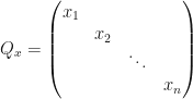
apply query matrix $Q_x$
apply some unitary $U$
measure in the standard basis

Since each of the answers reveal some property of $x$ , it is convenient to identify the collection of these properties with the question itself (I think of it as a “quantum Multiple Choice Question”, hence MCQ). Of course, not every collection of properties constitutes a valid quantum question — only those for which there exists a corresponding $|\psi\rangle$ and $U$ . (We will see some examples soon.)

MCQ algorithms

Simply put, an MCQ algorithm is a decision tree: each its leaf contains either 0 or 1 (the value of $f(x)$ for corresponding $x$ ), and each of the remaining nodes contains a quantum question and children correspond to answers.

Classical deterministic decision trees are very similar to MCQ algorithms, except that their nodes contain classical questions — at each node we can only ask one of the $n$ variables $x_i$ . Quantumly, we have a larger variety of questions — for example, we can ask XOR of two variables (as in Deutsch’s algorithm). Another difference is that a quantum question does not have a unique answer: if several answers are consistent with the input string $x$ , we will get one of them at random.

An obvious question regarding MCQ algorithms is this:

How can we exploit the quantum oracle to find $f(x)$ with less queries than classically?

Surprisingly, until recently essentially no other way of exploiting the quantum oracle was known, other than Deutsch’s XOR trick (see [MJM11] by Ashley Montanaro, Richard Jozsa, and Graeme Mitchison for more details). What is interesting about the [AIS13] paper is that it provides a new trick!

Query, measure, recurse!

All algorithms discussed in [AIS13] are MCQ and recursive. They proceed as follows:

query
measure
recurse

In the last step, depending on the measurement outcome, either $f(x)$ is found or the problem is reduced to a smaller instance and we proceed recursively. Let me explain how this works for two functions which I will call BALANCED and MAJORITY (they are special cases of EXACT and THRESHOLD discussed in [AIS13]).

BALANCED

$\mathrm{BALANCED}_{2k} (x_1, x_2, \dotsc, x_{2k}) = 1$ iff exactly $k$ of the variables $x_i$ are equal to 1. An MCQ algorithm asks a quantum question that can reveal the following properties of the input string $x$ :

$x$ is not balanced (the number of +1s and -1s is not equal)
$x_i$ is not equal to $x_j$ (for some $i \neq j$ )

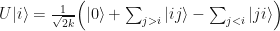
If we get the first answer then $\mathrm{BALANCED}_{2k}(x) = 0$ and we are done. If we get the second answer for some $i \neq j$ , we can ignore the variables $x_i$ and $x_j$ and recursively evaluate $\mathrm{BALANCED}_{2(k-1)}$ on the remaining variables. In total, we need at most $k$ queries (which can be shown to be optimal).

It remains to argue that the above is a valid quantum question. Alternatively, we can show how to prepare the following (unnormalized) quantum state:

$\sum_{i=1}^{2k} x_i |0\rangle + \sum_{i<j} (x_i - x_j) |ij\rangle$

(It lives in the space spanned by $|0\rangle$ and $|ij\rangle$ for all $i<j$ .) This can be easily done by taking

$|\psi\rangle = \sum_{i=0}^{2k} |i\rangle$

and $U$ that acts as

$U |i\rangle = \frac{1}{\sqrt{2k}} \Bigl( |0\rangle + \sum_{j>i} |ij\rangle - \sum_{j<i} |ji\rangle \Bigr)$

To check that $U$ is a valid isometry, notice that it maps $|i_1\rangle$ and $|i_2\rangle$ to paths that overlap in exactly one cell (rows are labeled by $i$ and columns by $j$ ):
Grid_paths
Since both states also have $|0\rangle$ in common, they are orthogonal.

MAJORITY

$\mathrm{MAJORITY}_{2k+1} (x_1, x_2, \dotsc, x_{2k+1}) = 1$ iff at least $k+1$ of the variables $x_i$ are equal to 1. This time the quantum question has answers

$x$ is not balanced when $x_i$ is omitted (for some $i$ )
$x_i$ is not equal to $x_j$ (for some $i \neq j$ )

If we get the first answer for some $i$ , we omit $x_i$ and any other variable. If we get the second answer for some $i \neq j$ , we ignore the variables $x_i$ and $x_j$ . In both cases we proceed by recursively evaluating $\mathrm{MAJORITY}_{2k-1}$ on the remaining variables. When only one variable is left, we query it to determine the answer. This requires at most $k+1$ queries in total (which again can be shown to be optimal).

The corresponding (unnormalized) state in this case is

$\sum_{i=1}^{2k+1} \sum_{j \neq i} x_i |j\rangle + \sqrt{2k-1} \sum_{i<j} (x_i - x_j) |ij\rangle$

(It lives in the space spanned by $|j\rangle$ for all $j$ and $|ij\rangle$ for all $i<j$ .) It can be obtained by choosing

$|\psi\rangle = \sum_{i=1}^{2k+1} |i\rangle$

and $U$ acting as

$U |i\rangle = \frac{1}{2k} \Bigl( \sum_{j \neq i} |j\rangle + \sqrt{2k-1} \sum_{j>i} |ij\rangle - \sqrt{2k-1} \sum_{j<i} |ji\rangle \Bigr)$

One can check that $U$ is an isometry using a similar picture as above.

Open questions

The problem of finding a quantum query algorithm with a given number of queries and a given success probability can be formulated as a semi-definite program. This was shown by Howard Barnum, Michael Saks, and Mario Szegedy in [BSS03] and can be used to obtain exact quantum query algorithms numerically. Unfortunately, this approach does not necessarily give any insight of why and how the obtained algorithm works. Nevertheless, it would be interesting to know if there is a similar simple characterization of MCQ algorithms.

The algorithms from [AIS13] described above are relatively simple. However, that does not mean that they were simple to find. In fact, the SDP corresponding to $\mathrm{BALANCED}_4$ had already been solved numerically in [MJM11]. Unfortunately, it did not provide enough insight to obtain an algorithm for $\mathrm{BALANCED}_{2k}$ for any $k$ . A similar situation is now with $\mathrm{EXACT}^6_{2,4}$ (which it is true if exactly two or four out of the six variables are true). From [MJM11] we know that it has an exact 3-query algorithm. Unfortunately, we do not have enough understanding to describe it in a simple way or generalize it. Besides, I wonder if $\mathrm{EXACT}^6_{2,4}$ has a 3-query MCQ algorithm, or do we actually need interference between the queries to find the answer so fast?

Finally, it would be interesting to know if there is any connection between exact quantum query algorithms and non-local games or Kochen–Specker type theorems.

Mamuta memuāri

math, music, me

Exact quantum query algorithms